Sales velocity

Sales velocity estimates how much revenue a qualified pipeline can produce per unit of time. It combines the number of qualified opportunities, average deal value, win rate, and average sales-cycle length.

The formula is:

Sales velocity = qualified opportunities x average deal value x win rate / average sales-cycle length

If cycle length is measured in days, the output is expected revenue per day. The result is a diagnostic estimate, not booked revenue or a commit forecast.

Why it matters

A sales pipeline can grow while expected revenue throughput stays flat. More opportunities may be offset by a lower win rate, smaller deals, or a longer cycle.

Sales velocity brings those four inputs into one model. It helps a team identify whether its main constraint is qualified pipeline volume, deal value, conversion, or time. That makes the metric more useful for diagnosis than a single blended pipeline total.

It also gives RevOps a consistent way to compare motions. Enterprise and SMB sales should normally have separate calculations because their deal values, win rates, and cycle lengths behave differently.

How it works

First, define a qualified opportunity. Do not count raw leads or every open CRM record.

Second, choose one segment and one measurement policy. The opportunity count, average deal value, win rate, and cycle length must describe the same motion.

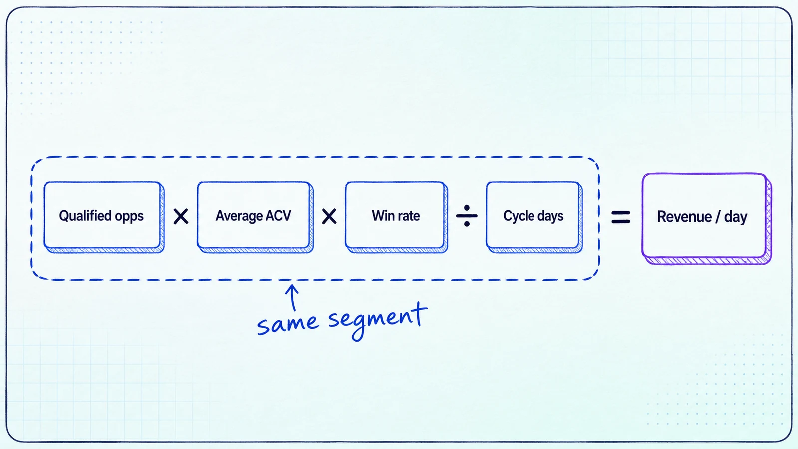
Formula diagram showing qualified opportunities, average ACV, win rate, and cycle days producing expected revenue per day. — Sales velocity is useful only when all four inputs describe the same sales motion.

Third, choose the deal-value basis. A SaaS team may use first-year ACV, but it should not mix ACV for some deals with total contract value for others.

Fourth, calculate win rate from the same qualified-opportunity population. If the denominator begins when an opportunity reaches a defined stage, cycle length should begin at that event too.

Fifth, calculate the average number of days from that start event to closed-won. The unit in the denominator determines the output unit.

The metric uses averages, so it does not model the timing and probability of each live deal. A stage-weighted forecast serves a different purpose.

SaaS example

Suppose one mid-market motion has:

40 qualified opportunities.
$18,000 average first-year ACV.
25% win rate.
60-day average sales cycle.

The calculation is:

40 x $18,000 x 0.25 / 60 = $3,000 per day

That result estimates expected revenue throughput under those assumptions. If win rate rises to 30% while the other inputs stay fixed, sales velocity rises to $3,600 per day.

The change does not prove that every current deal improved. It shows how one measured input changes the model.

Common mistakes

The first mistake is mixing segments, such as enterprise opportunity count with an SMB win rate.

The second is counting weak CRM records as qualified opportunities.

The third is changing the cycle start event between reports.

The fourth is treating the result as recognized revenue or a forecast commitment.

The fifth is trying to increase opportunity volume without checking its effect on win rate and cycle length.

Animation showing sales velocity rising from $3,000 to $3,600 per day when win rate increases from 25% to 30%. — With the same opportunities, ACV, and cycle length, a higher win rate increases expected revenue throughput.

How we see it

Sales velocity is most useful as a constraint finder. A lower result is not a diagnosis by itself. The team still needs to inspect which input moved and why.

Keep a separate velocity model for each meaningful segment, use the same definitions across reporting periods, and preserve the four underlying inputs. The combined number gives direction. The inputs tell an account executive or operator what to examine next.

Read the metric beside stage conversion and the sales funnel. That prevents a faster-looking average from hiding weaker qualification or a changed opportunity mix.